https://365datascience.com/linear-algebra-data-science/ -
If you’ve been researching or learning data science for a while, you must have stumbled upon linear algebra here and there. Linear algebra is an essential part of coding and thus: of data science and machine learning. But even then, you may be compelled to ask a question…
Why is Linear Algebra Actually Useful?
Linear algebra has tons of useful applications. However, in data science, there are several very important ones. So, in this tutorial, we will explore 3 of them:
- Vectorized code (a.k.a. array programming)
- Image recognition
- Dimensionality reduction
So, let’s start from the simplest and probably the most commonly used one – vectorized code.
Linear Algebra Applications: Vectorized Code (array programming)
We can certainly claim that the price of a house depends on its size. Suppose you know that the exact relationship for some neighborhood is given by the equation:
Price = 10190 + 223*size.
Moreover, you know the sizes of 5 houses: 693 sq.ft., 656 sq.ft., 1060 sq.ft., 487 sq.ft., and 1275 sq.ft.
So, what you want to do is plug-in each size in the equation and find the price of each house, right?
Well, for the first one we get: 10190 + 223*693 = 164729.
Then we can find the next one, and so on, until we find all prices.
Now, if we have 100 houses, doing that by hand would be quite tedious, wouldn’t it? Good thing we know how to code! One way to deal with that problem is by creating a loop. In Python that would look like:
house_sizes = [693, 656, 1060, 487, 1275]

for i in house_sizes:

price = 10190 + 223*i

print (price)
Iterating over the sizes, we can reach a satisfactory solution.
However, we could be even smarter than that, couldn’t we? What if we knew some linear algebra?
Let’s explore these two objects:
A (5×2) matrix and a (2×1) vector. The matrix contains a column of 1s and another – with the sizes of the houses.
M =
[table id=6 /]
The vector contains 10190 and 223 – the numbers from the equation.
V =
[table id=7 /]
Therefore, if we go about multiplying them, we will get a vector of length 5 ((5×2) * (2×1) = (5×1)). The first element will be equal to:
1*10190 + 693*223
The second to:
1*10190 + 656*223
And so on:
[table id=8 /]
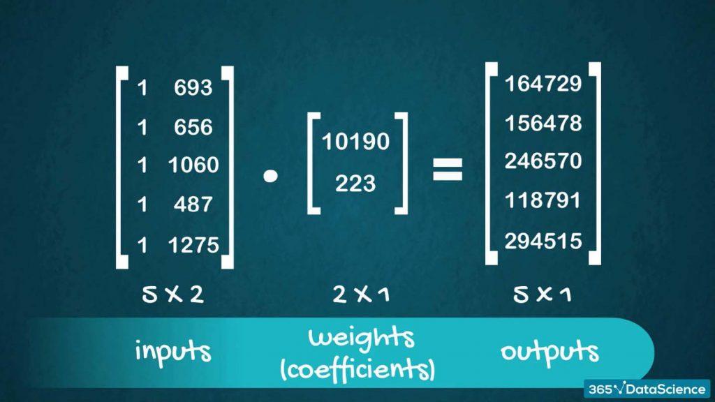 By inspecting these expressions, we quickly realize that the resulting vector contains all the manual calculations we tried to make earlier to find the prices.
Well, in machine learning and linear regressions in particular, this is exactly how algorithms work. We’ve got an inputs matrix; a weights, or a coefficients matrix; and an output matrix.
Without diving too deep into the mechanics of it here, let’s note something.
If we have 10,000 inputs, the initial matrix would be (10000×2), right? But the weights matrix would still be 2×1. So, when we multiply them, the resulting output matrix would be 10000×1. This shows us that regardless of the number of inputs, we will get just as many outputs. Moreover, the equation doesn’t change, as it only contained the two coefficients – 10190 and 223.
This concept is of paramount importance to machine learning, precisely because of its generality.
So, whenever we are using linear algebra to compute many values simultaneously, we call this ‘array programming’ or ‘vectorized code’. It turns out that vectorized code is much, much faster (than loops for instance). There are libraries such as NumPy that are optimized for performing this kind of operations which greatly increases the computational efficiency of our code.
Linear Algebra Applications: What About Image recognition?
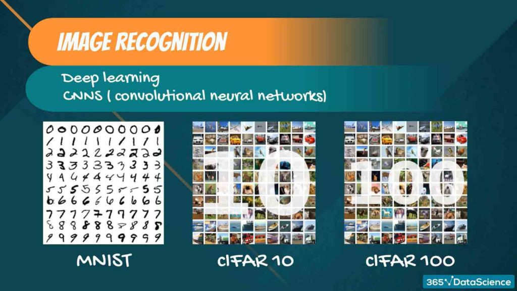
In the last few years, deep learning, and deep neural networks specifically, conquered image recognition. On the forefront are convolutional neural networks or CNNs in short. But what is the basic idea? Well, you can take a photo, feed it to the algorithm and classify it. Famous examples are:
- the MNIST dataset, where the task is to classify handwritten digits
- CIFAR-10, where the task is to classify animals and vehicles
and
- CIFAR-100, where you have 100 different classes of images
The main problem is that we cannot just take a photo and give it to the computer.
Therefore, we must design a way to turn that photo into numbers in order to communicate the image to the computer.
Here’s where linear algebra comes in.
Each photo has some dimensions, right? Say, this photo is 400×400 pixels. Each pixel in a photo is basically a colored square. Given enough pixels and a big enough zoom-out causes our brain to perceive this as an image, rather than a collection of squares.
Let’s dig into that. Here’s a simple greyscale photo. The greyscale contains 256 shades of grey, where 0 is totally white and 255 is totally black, or vice versa.
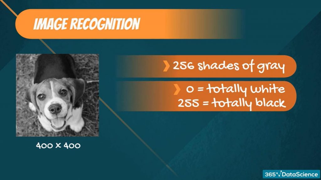
In fact, we can express this photo as a matrix. If the photo is 400×400, then that’s a 400×400 matrix. Each element of that matrix is a number from 0 to 255. It shows the intensity of the color grey in that pixel.
That’s how the computer ‘sees’ a photo.
But greyscale is boring, isn’t it? What about colored photos?
Well, so far, we had two dimensions – width and height, while the number inside corresponded to the intensity of color. What if we want more colors?
Now, one solution mankind has come up with is the RGB scale, where RGB stands for red, green, and blue. The idea is that any color, perceivable by the human eye can be decomposed into some combination of red, green, and blue, where the intensity of each color is from 0 to 255 – a total of 256 shades.
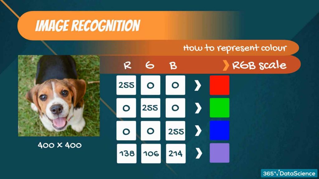
So, in order to represent a colored photo in some linear algebraic form, we must take the example from before and add another dimension – color.
Hence, instead of a 400×400 matrix, we get a 3x400x400 tensor!
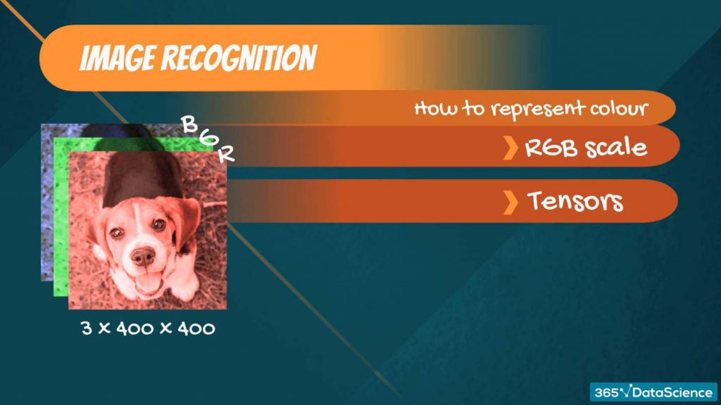
This tensor contains three 400×400 matrices. One for each color – red, green, and blue.
And that’s how deep neural networks work with photos!
Linear Algebra Applications: Dimensionality Reduction
Assuming we haven’t seen eigenvalues and eigenvectors ever before, there is not much to say here, except for developing some intuition.
Imagine we have a dataset with 3-variables. Visually, our data may look like this. In order to represent each of those points, we have used 3 values – one for each variable x, y, and z. Therefore, we are dealing with an m-by-3 matrix. So, the point “i” corresponds to a vector X i, y i, and z i.
Note that those three variables: x, y, and z are the three axes of this plane.
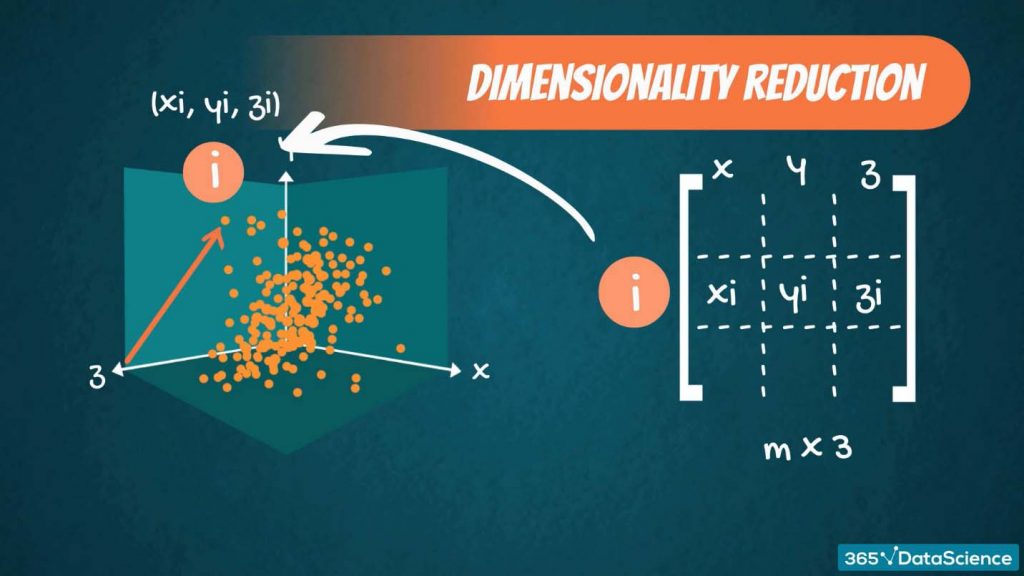
Here’s where it becomes interesting.
In some cases, we can find a plane very close to the data. Something like this.
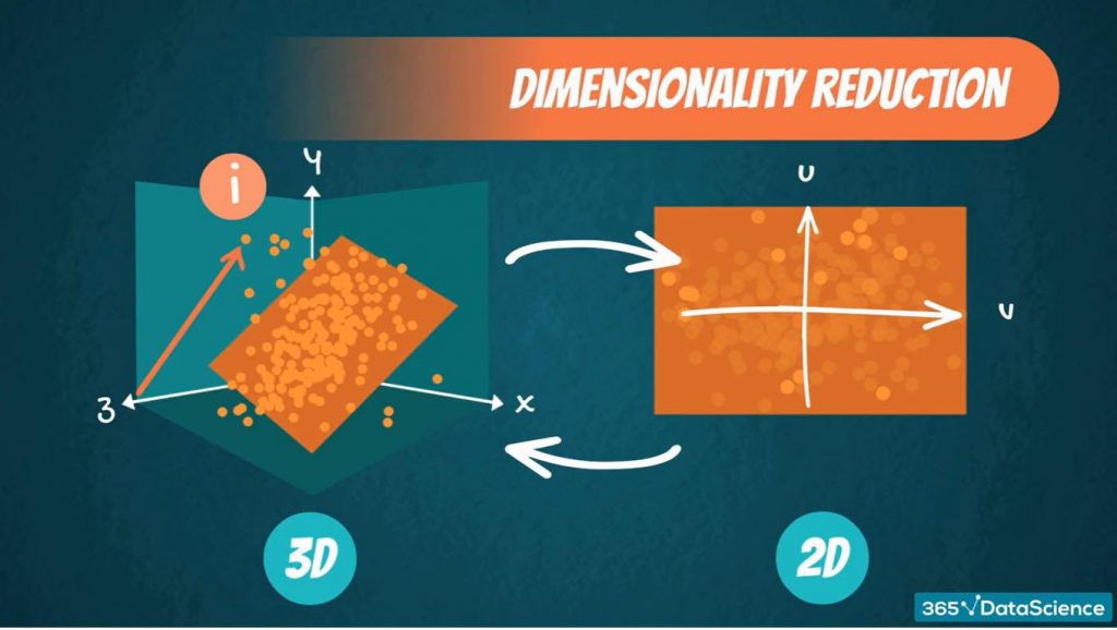
This plane is two-dimensional, so it is defined by two variables, say u and v. Not all points lie on this plane, but we can approximately say that they do.
And linear algebra provides us with fast and efficient ways to transform our initial matrix from mx3, where the three variables are x, y, and z, into a new matrix, which is mx2, where the two variables are u and v.
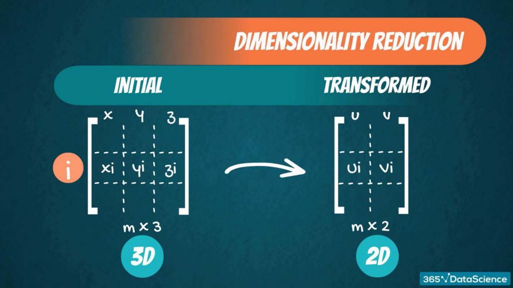
So, this way, instead of having 3 variables, we reduce the problem to 2 variables.
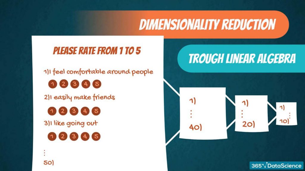
In fact, if you have 50 variables, you can reduce them to 40, or 20, or even 10.
But how does that relate to the real world? Why does it make sense to do that?
Well, imagine a survey where there is a total of 50 questions. Three of them are the following:
Please rate from 1 to 5:
- I feel comfortable around people
- I easily make friends
and
- I like going out
Well, these questions may seem different, but in the general case, they aren’t. They all measure your level of extroversion. So, it makes sense to combine them, right? That’s where dimensionality reduction techniques and linear algebra come in! Very, very often we have too many variables that are not so different, so we want to reduce the complexity of the problem by reducing the number of variables.
Some Final Words…
While there are many different ways in which linear algebra helps us in data science, these 3 are paramount to topics that we cover in The 365 Data Science Program. So, feel free to read more about these use cases in our Linear Regression, PCA , and Neural Networks blog posts!
Ready to take the next step towards a data science career?
Check out the complete Data Science Program today. Start with the fundamentals with our Statistics, Maths, and Excel courses. Build up a step-by-step experience with SQL, Python, R, and Tableau. And upgrade your skillset with Machine Learning, Deep Learning, Credit Risk Modeling, Time Series Analysis, and Customer Analytics in Python. Still not sure you want to turn your interest in data science into a career? We also offer a free preview version of the Data Science Program. You’ll receive 12 hours of beginner to advanced content for free. It’s a great way to see if the program is right for you.
#Python
#365datascience #DataScience #data #science #365datascience #BigData #tutorial #infographic #career #salary #education #howto #scientist #engineer #course #engineer #MachineLearning #machine #learning #certificate #udemy

No comments:
Post a Comment