https://365datascience.com/moving-average-model/ -

What do we use the Moving Average model for?
In time-series, we sometimes observe similarities between past errors and present values. That’s because certain unpredictable events happen, and they need to be accounted for.
In other words, by knowing how far off our estimation yesterday was, compared to the actual value, we can tweak our model, so that it responds accordingly.
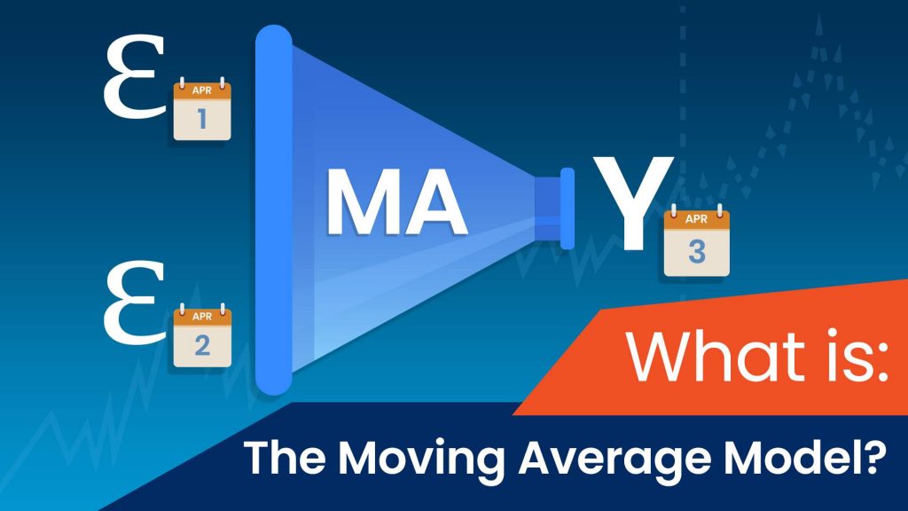
So, in this tutorial, we’re going to examine a model that considers past residuals – the Moving Average model. We’ll discuss notation, learn how to interpret it and then digest the different parts.
Let’s get right down to it!
What is the equation of a Moving Average model?
Let’s suppose that “r” is some time-series variable, like returns. Then, a simple Moving Average (MA) model looks like this:
rt = c + θ1 ϵt-1 + ϵt
Now, just like we did in the tutorial about the Autoregressive model, let’s go over the different parts of this equation. This will ensure you understand the idea thoroughly.
What is rt?
For starters, rt represents the values of “r” in the current period – t. In terms of returns, it’s what we’re estimating the returns for today will be.
What is c?
The first thing we see on the right side of the model is “c” – this stands for a constant factor. Of course, this is just the general representation and we would substitute this with a numeric value when we’re actually modeling data.
What is θ_1?
Next, θ1 is a numeric coefficient for the value associated with the 1st lag. We prefer not to use ϕ1 like in the Autoregressive model, to avoid confusion.
What is ϵtand ϵt-1?
Then come ϵt and ϵt-1 which represent the residuals for the current and the previous period, respectively.
For anybody not familiar with the term, a residual is the same as an error term – it expresses the difference between the observed value for a variable and our estimation. In this specific case: ϵt-1 = rt-1 – r̂t-1 , where r̂t-1 represents our estimation for the previous period.
So, how do we generate these residuals?
It’s quite simple. We start from the beginning of the dataset r1 and try to predict each value (r̂2, r̂3, etc). Depending on how far off we were each time, we get a residual ϵt = rt – r̂t. Therefore, we generate these residuals as we go through the set and create the ϵ variable as we move through time (from period 1, all the way up to the current period).
What are the similarities between the Moving Average model and the Autoregressive model?
You can notice some parallels between the Moving Average model and the Autoregressive model we examined in a previous article. In fact, we can say a simple moving average model is equivalent to an infinite-lag autoregressive model with certain restrictions. You can find more details on that here.
Not to mention that an inverse relationship exists as well. To be more precise, a simple Autoregressive model can be a close approximator to an infinite-lag moving average model. If you’re interested to learn more, you can read about it here.
Now, in both models, we have the present-day value r_t equal a sum of a constant c; some error term ϵ_t; and a lagged value (rt-1, ϵt-1) multiplied by an assigned coefficient (ϕ1, θ1). The only major difference is that the autoregressive model uses the value of the variable (rt-1), while the moving average model relies on the residual (ϵt-1).
Finally, there’s one more common trait of the AR and MA models – the restriction remains that the absolute value of each coefficient should be less than 1(|ϕn|< θn|<1). Once again, this is to prevent compounded effects exploding in magnitude, as we discussed in the AR model tutorial.
What is the difference between the Moving Average model and the Autoregressive model?
Apart from sharing a lot of similarities, the two types of models also have several key differences. One such distinction between them comes in the form of determining the maximum amounts of lags we are willing to include in our model. While with the Autoregressive model we relied on the Partial Autocorrelation Function, a.k.a the PACF, with Moving Averages we rely on the Autocorrelation Function or the ACF for short.
The reason is that MA models aren’t based on past period returns. Therefore, determining which lagged values have a significant direct effect on the present-day ones is not relevant.
Anyways, the total accumulated effects accommodate for these unexpected shocks. Hence, the ACF plot provides us with information on how many lags our model should use.
If you want to learn more about the ACF, PACF and how to determine the right, check out the 365 Data Science program. You’ll learn the most important models for Time Series Analysis, like the AR and the MA and how to apply them in Python!
Want to explore the curriculum or sign up 12 hours of beginner to advanced video content for free? Click on the button below.
#Python
#365datascience #DataScience #data #science #365datascience #BigData #tutorial #infographic #career #salary #education #howto #scientist #engineer #course #engineer #MachineLearning #machine #learning #certificate #udemy
No comments:
Post a Comment